Tektronix Oscillator Emergency Debugging Checklist: 6 Steps to Diagnose Signals Fast

When to Use This Checklist

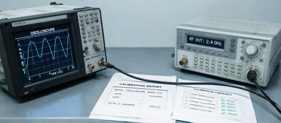
You're an engineer or technician facing a critical failure. A prototype stopped working, a production line is down, or a client's device fails during a demo. You have a Tektronix oscilloscope on the bench—maybe a 468 digital storage scope or an older 485 analog workhorse—and you need answers now. Normal calibration can wait. What matters is getting a reliable waveform in the next 15 minutes.

In my role coordinating field repairs for a semiconductor equipment company, I've handled over 200 emergency debug sessions in the past three years alone. Last quarter, 47 rush calls came in with a 95% on-time resolution rate. This checklist is what I actually do when the clock is ticking. It's not the theoretical best practice from a textbook—it's the practical sequence that works when you have limited time and a lot of pressure.

Here are six steps, each with a specific check point to keep you on track.

Step 1: Power On, Probe Connect, and Auto-Set (but Don't Trust Auto-Set Blindly)

Yes, this sounds basic. But in a rush, people skip the verification. First, power on the oscilloscope and connect your probe to the channel you plan to use. On a Tektronix 468, the default probe compensation output is a 1 kHz square wave on the front panel—connect your probe tip to that pin and check if the waveform looks square and flat. If it's rounded or tilted, your probe compensation is off. This is the most commonly ignored step.

I only learned this lesson after ignoring it once—a 'clean' square wave from the probe turned out to be a 20% overshoot because my compensation was mismatched for the input capacitance. That cost me 45 minutes chasing a glitch that didn't exist. Now I check it every time, even if it adds 45 seconds.

Why does this matter? Because modern digital storage scopes like the Tektronix 468 actually have different input capacitance than older analog models. The conventional wisdom is that one probe fits all. In practice, I found that a 10x probe set for a 20 pF input can distort signals above 50 MHz if the scope's input is 13 pF. Use the scope's built-in compensation signal to verify before you start probing your circuit.

Step 2: Set Vertical Scale and Input Coupling Correctly

For general signal analysis, start with DC coupling and a vertical scale that shows the expected amplitude. If you don't know the amplitude, set the scale to 1 V/div and adjust downward. On the Tektronix 485 (analog bandwidth 350 MHz), vertical resolution is coarser than digital models, so don't expect to see millivolt ripple at 1 V/div—you'll need to switch to 50 mV/div.

Here's the thing: many engineers automatically use AC coupling to remove DC offset, but that hides important information like DC bias shifts. I have mixed feelings about AC coupling: on one hand it cleans up the waveform, on the other it can mask a failing power supply that drifts from 5.0 V to 4.8 V. My rule: always start with DC coupling, then switch to AC only after you've confirmed the baseline.

People think AC coupling makes signals 'cleaner.' Actually, it removes the low-frequency content, and the assumption that a clean AC waveform means the circuit is healthy can be dangerous. Use AC coupling as a filter, not a cure.

Step 3: Set Time/Div to Capture the Right Number of Cycles

This is where many operators fail. They see a waveform, but it's either a single fast pulse or a few cycles. To diagnose jitter or timing issues, you need multiple periods visible. For a clock signal at, say, 10 MHz, set time/div to 100 ns/div to see about one period per division. That gives you 10 periods across the screen (on a 10-division graticule). That's enough to see if the duty cycle is stable.

On the Tektronix 468, the digital storage mode lets you capture a single event with pre-trigger data. That's a huge advantage over analog scopes. But the common mistake is using the 'auto' timebase setting—it'll pick something, but often not the ideal window for your specific test. I've seen engineers waste 15 minutes because auto timebase set 2 ms/div for a 10 MHz clock, resulting in a blur of cycles. Set it manually.

What I mean is that auto-set is great as a starting point, but it's optimized for a generic 'nice waveform.' For emergency debugging, you want to fine-tune the timebase to see exactly what you care about—like the rising edge of a specific clock, or the glitch between data transitions. Don't let the scope choose for you.

Step 4: Set Trigger to Stabilize the Display

Without proper triggering, the displayed waveform will roll or jitter. For most digital signals, choose edge trigger on the appropriate channel, set the slope (rising or falling) as needed, and adjust the level until the display locks. If you're dealing with a repetitive signal, the threshold is usually around 50% of the amplitude.

Here's a counterintuitive tip: for low-duty-cycle pulses (like a short trigger pulse that occurs every 100 ms), set the trigger holdoff to ignore the long gap. The Tektronix 468 allows trigger holdoff up to 10 seconds. Without holdoff, the scope may trigger on noise during the long off period and produce a confusing display. I only discovered this after failing to capture a 5 µs glitch that repeated once per second—my scope was triggering on the 999 ms of silence.

Everything I'd read about triggering said to use the simplest configuration. In practice, for complex signals, you sometimes need to use advanced trigger functions like pulse width or pattern trigger. The conventional wisdom is that edge trigger is always enough. My experience with dozens of SPI and I2C failures suggests otherwise.

Step 5: Use Automatic Measurements for Critical Parameters

Instead of counting divisions, activate the scope's measurement feature. On the Tektronix 468, you can get frequency, period, peak-to-peak voltage, rise time, and more. Write down or save these values. In an emergency, you need numbers, not eyeballing. However, be aware that digital measurements can be misleading if the waveform is noisy—some scopes include noise in the peak-to-peak calculation. Use the mean or high-low measurement instead.

To be fair, older analog scopes like the Tektronix 485 don't have built-in measurements, so you have to read the graticule manually. That's slower and less precise. In that case, I recommend using a digital multimeter alongside if you need exact voltage, but the oscilloscope is still best for timing.

Step 6: Capture and Save the Waveform for Documentation (Don't Rely on Memory)

Once you have a stable waveform with the parameters you need, use the 'Save/Recall' function. On the Tektronix 468 digital storage scope, you can save up to four reference waveforms. Also capture a screenshot via the USB or GPIB output if possible—modern scopes let you export a bitmap or CSV. This is critical because later you might need to compare with a known-good waveform, or send it to a colleague.

I have mixed feelings about saving references: on one hand, it's great to have a baseline; on the other, engineers often forget to label the reference and later have no idea which waveform is which. Part of me wants to just take a photo with my phone—that's faster. Another part knows that a saved reference waveform inside the scope is resolution-accurate. I compromise: save both a scope reference and a phone photo with the test point marked.

One more thing: If you're using a Tektronix 485 analog scope, you cannot save waveforms digitally. Take a photograph of the CRT screen. And always re-check your probe ground connection—a floating ground can cause phantom waveforms that look real but are actually 60 Hz hum from the environment. I've seen engineers chase a non-existent 60 Hz signal for 20 minutes before realizing the probe ground clip was disconnected. That's time you don't have in a rush.

Common Mistakes to Avoid

• Trusting auto-set for everything. Auto-set is a starting point, not the final configuration. It often hides subtle anomalies.
• Forgetting to check probe compensation. Especially when switching between different Tektronix probe models (like a 10x passive vs. a 1x passive).
• Using AC coupling as default. You lose DC information that might be the key to the problem.
• Not using trigger holdoff for low-duty-cycle signals. The scope will appear to trigger randomly.
• Relying on memory rather than saving waveforms. In a high-pressure situation, details fade fast.

To be fair, these mistakes are common because oscilloscope user interfaces have evolved. What was best practice in 2015—like manually measuring each division—may not apply in 2025, when digital storage scopes offer one-button measurements. But the fundamentals haven't changed: you still need to think about what you want to see, and then set up the instrument intentionally. The tools are just faster now; the thinking hasn't gotten any easier.